Gaussian-binary restricted Boltzmann machine on a 2D linear mixture.
Example for Gaussian-binary restricted Boltzmann machine used for blind source separation on a linear 2D mixture.
Theory
The results are part of the publication Gaussian-binary restricted Boltzmann machines for modeling natural image statistics. Melchior, J., Wang, N., & Wiskott, L.. (2017). PLOS ONE, 12(2), 1–24. .
If you are new on GRBMs, you can have a look into my master’s theses
See also ICA_2D_example
Results
The code given below produces the following output.
Visualization of the weight vectors learned by the GRBM with 4 hidden units together with the contour plot of the learned probability density function (PDF).
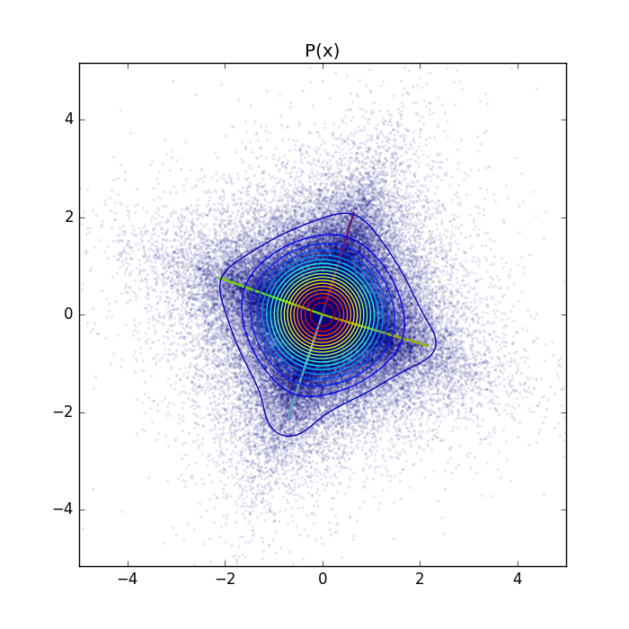
For a better visualization also the log-PDF.

The parameters values and the component scaling values P(h_i) are as follows:
Weigths:
[[-2.13559806 -0.71220501  0.64841691  2.17880554]
 [ 0.75840129 -2.13979672  2.09910978 -0.64721076]]
Visible bias:
[[ 0.  0.]]
Hidden bias:
[[-7.87792514 -7.60603139 -7.73935758 -7.722771  ]]
Sigmas:
[[ 0.74241256  0.73101419]]

Scaling factors:
P(h_0) [[ 0.83734074]]
P(h 1 ) [[ 0.03404849]]
P(h 2 ) [[ 0.04786942]]
P(h 3 ) [[ 0.0329518]]
P(h 4 ) [[ 0.04068302]]
The exact log-likelihood, annealed importance sampling estimation, and reverse annealed importance sampling estimation for training and test data are:
True log partition:   1.40422867085  ( LL_train:  -2.74117592643 , LL_test:  -2.73620936613  )
AIS  log partition:   1.40390312781  ( LL_train:  -2.74085038339 , LL_test:  -2.73588382309  )
rAIS  log partition:  1.40644042744  ( LL_train:  -2.74338768302 , LL_test:  -2.73842112273  )
For comparison here is the original mixing matrix an the corresponding ICA estimation.

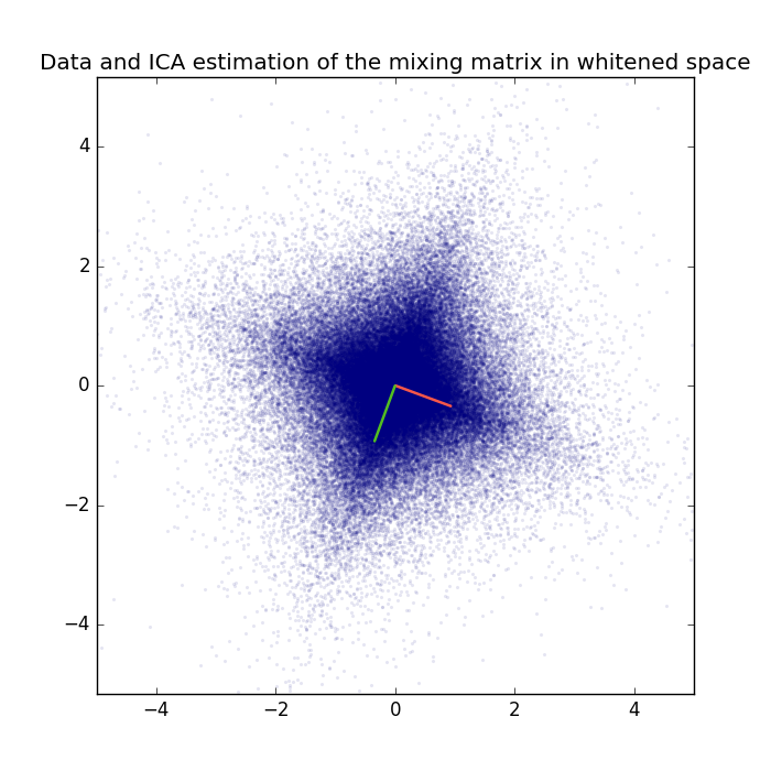
The exact log-likelihood for ICA is almost the same as that for the GRBM with 4 hidden units.
ICA log-likelihood on train data: -2.74149951412
ICA log-likelihood on test data:  -2.73579105422
We can also calculate the Amari distance between true mixing , the ICA estimation, and the GRBM estimation. Since the GRBM has learned 4 weight vectors we calculate teh Amari distance between the true mixing matrix and all sets of 2 weight-vectors of the GRBM.
Amari distance between true mixing matrix and ICA estimation:             0.00621143307663
Amari distance between true mixing matrix and GRBM weight vector 1 and 2: 0.0292827450487
Amari distance between true mixing matrix and GRBM weight vector 1 and 3: 0.0397992351592
Amari distance between true mixing matrix and GRBM weight vector 1 and 4: 0.336416964036
Amari distance between true mixing matrix and GRBM weight vector 2 and 3: 0.435997388341
Amari distance between true mixing matrix and GRBM weight vector 2 and 4: 0.0557649366433
Amari distance between true mixing matrix and GRBM weight vector 3 and 4: 0.0666442992135
Weight-vectors 1 and 4 as well as 2 and 3 are almost 180 degrees rotated version of each other, which can also be seen from the weight matrix values given above and thus the Amari distance to the mixing matrix is high.
For a real-world application see the GRBM_natural_images example.
Source code
""" Toy example using GB-RBMs on a blind source seperation toy problem.

    :Version:
        1.1.0

    :Date:
        28.04.2017

    :Author:
        Jan Melchior

    :Contact:
        JanMelchior@gmx.de

    :License:

        Copyright (C) 2017 Jan Melchior

        This file is part of the Python library PyDeep.

        PyDeep is free software: you can redistribute it and/or modify
        it under the terms of the GNU General Public License as published by
        the Free Software Foundation, either version 3 of the License, or
        (at your option) any later version.

        This program is distributed in the hope that it will be useful,
        but WITHOUT ANY WARRANTY; without even the implied warranty of
        MERCHANTABILITY or FITNESS FOR A PARTICULAR PURPOSE.  See the
        GNU General Public License for more details.

        You should have received a copy of the GNU General Public License
        along with this program.  If not, see <http://www.gnu.org/licenses/>.

"""

# Import numpy, numpy extensions
import numpy as numx
import pydeep.base.numpyextension as numxext

# Import models, trainers and estimators
import pydeep.rbm.model as model
import pydeep.rbm.trainer as trainer
import pydeep.rbm.estimator as estimator

# Import linear mixture, preprocessing, and visualization
from pydeep.misc.toyproblems import generate_2d_mixtures
import pydeep.preprocessing as pre
import pydeep.misc.visualization as vis

numx.random.seed(42)

# Create a 2D mxiture
data, mixing_matrix = generate_2d_mixtures(100000, 1, 1.0)

# Whiten data
zca = pre.ZCA(data.shape[1])
zca.train(data)
whitened_data = zca.project(data)

# split training test data
train_data = whitened_data[0:numx.int32(whitened_data.shape[0] / 2.0), :]
test_data = whitened_data[numx.int32(whitened_data.shape[0] / 2.0
                                     ):whitened_data.shape[0], :]

# Input output dims
h1 = 2
h2 = 2
v1 = whitened_data.shape[1]
v2 = 1

# Create model
rbm = model.GaussianBinaryVarianceRBM(number_visibles=v1 * v2,
                                      number_hiddens=h1 * h2,
                                      data=train_data,
                                      initial_weights='AUTO',
                                      initial_visible_bias=0,
                                      initial_hidden_bias=0,
                                      initial_sigma=1.0,
                                      initial_visible_offsets=0.0,
                                      initial_hidden_offsets=0.0,
                                      dtype=numx.float64)

# Set the hidden bias such that the scaling factor is 0.1
rbm.bh = -(numxext.get_norms(rbm.w + rbm.bv.T, axis=0) - numxext.get_norms(
    rbm.bv, axis=None)) / 2.0 + numx.log(0.1)
rbm.bh = rbm.bh.reshape(1, h1 * h2)

# Create trainer
trainer_cd = trainer.CD(rbm)

# Hyperparameters
batch_size = 1000
max_epochs = 50
k = 1
epsilon = [1,0,1,0.1]

# Train model
print 'Training'
print 'Epoch\tRE train\tRE test \tLL train\tLL test '
for epoch in range(1, max_epochs + 1):

    # Shuffle data points
    train_data = numx.random.permutation(train_data)

    # loop over batches
    for b in range(0, train_data.shape[0] / batch_size):
        trainer_cd.train(data=train_data[b:(b + batch_size), :],
                         num_epochs=1,
                         epsilon=epsilon,
                         k=k,
                         momentum=0.0,
                         reg_l1norm=0.0,
                         reg_l2norm=0.0,
                         reg_sparseness=0.0,
                         desired_sparseness=0.0,
                         update_visible_offsets=0.0,
                         update_hidden_offsets=0.0,
                         restrict_gradient=False,
                         restriction_norm='Cols',
                         use_hidden_states=False,
                         use_centered_gradient=False)

    # Calculate Log likelihood and reconstruction error
    RE_train = numx.mean(estimator.reconstruction_error(rbm, train_data))
    RE_test = numx.mean(estimator.reconstruction_error(rbm, test_data))
    logZ = estimator.partition_function_factorize_h(rbm, batchsize_exponent=h1)
    LL_train = numx.mean(estimator.log_likelihood_v(rbm, logZ, train_data))
    LL_test = numx.mean(estimator.log_likelihood_v(rbm, logZ, test_data))
    print '%5d \t%0.5f \t%0.5f \t%0.5f \t%0.5f' % (epoch,
                                                   RE_train,
                                                   RE_test,
                                                   LL_train,
                                                   LL_test)

# Calculate partition function and its AIS approximation
logZ = estimator.partition_function_factorize_h(rbm, batchsize_exponent=h1)
logZ_AIS = estimator.annealed_importance_sampling(rbm,
                                                  num_chains=100,
                                                  k=1,
                                                  betas=1000,
                                                  status=False)[0]
logZ_rAIS = estimator.reverse_annealed_importance_sampling(rbm,
                                                  num_chains=100,
                                                  k=1,
                                                  betas=1000,
                                                  status=False)[0]

# Calculate and print LL
print("")
print("\nTrue log partition: ", logZ, " ( LL_train: ", numx.mean(
    estimator.log_likelihood_v(
        rbm, logZ, train_data)), ",", "LL_test: ", numx.mean(
    estimator.log_likelihood_v(rbm, logZ, test_data)), " )")
print("\nAIS  log partition: ", logZ_AIS, " ( LL_train: ", numx.mean(
    estimator.log_likelihood_v(
        rbm, logZ_AIS, train_data)), ",", "LL_test: ", numx.mean(
    estimator.log_likelihood_v(rbm, logZ_AIS, test_data)), " )")
print("\nrAIS  log partition: ", logZ_rAIS, " ( LL_train: ", numx.mean(
    estimator.log_likelihood_v(
        rbm, logZ_rAIS, train_data)), ",", "LL_test: ", numx.mean(
    estimator.log_likelihood_v(rbm, logZ_rAIS, test_data)), " )")
print("")
# Print parameter
print '\nWeigths:\n', rbm.w
print 'Visible bias:\n', rbm.bv
print 'Hidden bias:\n', rbm.bh
print 'Sigmas:\n', rbm.sigma
print

# Calculate P(h) wich are the scaling factors of the Gaussian components
h_i = numx.zeros((1, h1 * h2))
print("Scaling factors:")
print 'P(h_0)', numx.exp(rbm.log_probability_h(logZ, h_i))
for i in range(h1 * h2):
    h_i = numx.zeros((1, h1 * h2))
    h_i[0, i] = 1
    print 'P(h', (i + 1), ')', numx.exp(rbm.log_probability_h(logZ, h_i))
print


# Independent Component Analysis (ICA)
ica = pre.ICA(train_data.shape[1])
ica.train(train_data, iterations=100,status=False)
data_ica = ica.project(train_data)

# Print ICA log-likelihood
print("ICA log-likelihood on train data: " + str(numx.mean(
    ica.log_likelihood(data=train_data))))
print("ICA log-likelihood on test data: " + str(numx.mean(
    ica.log_likelihood(data=test_data))))
print("")

# Print Amari distances
print("Amari distanca between true mixing matrix and ICA estimation: "+str(
    vis.calculate_amari_distance(zca.project(mixing_matrix.T), ica.projection_matrix.T)))

print("Amari distanca between true mixing matrix and GRBM weight vector 1 and 2: "+str(
    vis.calculate_amari_distance(zca.project(mixing_matrix.T),
                                 numx.vstack((rbm.w.T[0:1],rbm.w.T[1:2])))))

print("Amari distanca between true mixing matrix and GRBM weight vector 1 and 3: "+str(
    vis.calculate_amari_distance(zca.project(mixing_matrix.T),
                                 numx.vstack((rbm.w.T[0:1],rbm.w.T[2:3])))))

print("Amari distanca between true mixing matrix and GRBM weight vector 1 and 4: "+str(
    vis.calculate_amari_distance(zca.project(mixing_matrix.T),
                                 numx.vstack((rbm.w.T[0:1],rbm.w.T[3:4])))))

print("Amari distanca between true mixing matrix and GRBM weight vector 2 and 3: "+str(
    vis.calculate_amari_distance(zca.project(mixing_matrix.T),
                                 numx.vstack((rbm.w.T[1:2],rbm.w.T[2:3])))))

print("Amari distanca between true mixing matrix and GRBM weight vector 2 and 4: "+str(
    vis.calculate_amari_distance(zca.project(mixing_matrix.T),
                                 numx.vstack((rbm.w.T[1:2],rbm.w.T[3:4])))))

print("Amari distanca between true mixing matrix and GRBM weight vector 3 and 4: "+str(
    vis.calculate_amari_distance(zca.project(mixing_matrix.T),
                                 numx.vstack((rbm.w.T[2:3],rbm.w.T[3:4])))))

# Display results
# create a new figure of size 5x5
vis.figure(0, figsize=[7, 7])
vis.title("P(x)")
# plot the data
vis.plot_2d_data(whitened_data)
# plot weights
vis.plot_2d_weights(rbm.w, rbm.bv)
# pass our P(x) as function to plotting function
vis.plot_2d_contour(lambda v: numx.exp(rbm.log_probability_v(logZ, v)))
# No inconsistent scaling
vis.axis('equal')
# Set size of the plot
vis.axis([-5, 5, -5, 5])

# Do the sam efor the LOG-Plot
# create a new figure of size 5x5
vis.figure(1, figsize=[7, 7])
vis.title("Ln( P(x) )")
# plot the data
vis.plot_2d_data(whitened_data)
# plot weights
vis.plot_2d_weights(rbm.w, rbm.bv)
# pass our P(x) as function to plotting function
vis.plot_2d_contour(lambda v: rbm.log_probability_v(logZ, v))
# No inconsistent scaling
vis.axis('equal')
# Set size of the plot
vis.axis([-5, 5, -5, 5])

# Figure 2 - Data and mixing matrix in whitened space
vis.figure(3, figsize=[7, 7])
vis.title("Data and mixing matrix in whitened space")
vis.plot_2d_data(whitened_data)
vis.plot_2d_weights(numxext.resize_norms(zca.project(mixing_matrix.T).T,
                                         norm=1,
                                         axis=0))
vis.axis('equal')
vis.axis([-5, 5, -5, 5])

# Figure 3 - Data and ica estimation of the mixing matrix in whitened space
vis.figure(4, figsize=[7, 7])
vis.title("Data and ICA estimation of the mixing matrix in whitened space")
vis.plot_2d_data(whitened_data)
vis.plot_2d_weights(numxext.resize_norms(ica.projection_matrix,
                                         norm=1,
                                         axis=0))
vis.axis('equal')
vis.axis([-5, 5, -5, 5])

vis.show()