Principal Component Analysis on a 2D example.

Example for Principal Component Analysis (PCA) on a linear 2D mixture.

Theory

If you are new on PCA, a good theoretical introduction is given by the Course Material in combination with the following video lectures.

Results

The code given below produces the following output.

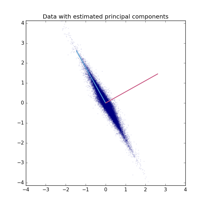
The data is plotted with the extracted principal components.

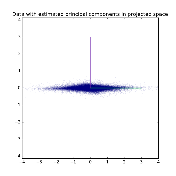
Data and extracted principal components can also be plotted in the projected space.

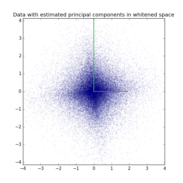
The PCA-class can also perform whitening. Data and extracted principal components are plotted in the whitened space.

For a real-world application see the PCA_eigenfaces example.

Source code

""" Example for the Principal Component Analysis on a 2D example.

    :Version:
        1.1.0

    :Date:
        22.04.2017

    :Author:
        Jan Melchior

    :Contact:
        JanMelchior@gmx.de

    :License:

        Copyright (C) 2017 Jan Melchior

        This file is part of the Python library PyDeep.

        PyDeep is free software: you can redistribute it and/or modify
        it under the terms of the GNU General Public License as published by
        the Free Software Foundation, either version 3 of the License, or
        (at your option) any later version.

        This program is distributed in the hope that it will be useful,
        but WITHOUT ANY WARRANTY; without even the implied warranty of
        MERCHANTABILITY or FITNESS FOR A PARTICULAR PURPOSE.  See the
        GNU General Public License for more details.

        You should have received a copy of the GNU General Public License
        along with this program.  If not, see <http://www.gnu.org/licenses/>.
"""

# Import numpy, numpy extensions, PCA, 2D linear mixture, and visualization module
import numpy as numx
from pydeep.preprocessing import PCA
from pydeep.misc.toyproblems import generate_2d_mixtures
import pydeep.misc.visualization as vis

# Set the random seed
# (optional, if stochastic processes are involved we get the same results)
numx.random.seed(42)

# Create 2D linear mixture, 50000 samples, mean = 0, std = 3
data, _ = generate_2d_mixtures(num_samples=50000,
                               mean=0.0,
                               scale=3.0)

# PCA
pca = PCA(data.shape[1])
pca.train(data)
data_pca = pca.project(data)

# Display results

# For better visualization the principal components are rescaled
scale_factor = 3

# Figure 1 - Data with estimated principal components
vis.figure(0, figsize=[7, 7])
vis.title("Data with estimated principal components")
vis.plot_2d_data(data)
vis.plot_2d_weights(scale_factor*pca.projection_matrix)
vis.axis('equal')
vis.axis([-4, 4, -4, 4])

# Figure 2 - Data with estimated principal components in projected space
vis.figure(2, figsize=[7, 7])
vis.title("Data with estimated principal components in projected space")
vis.plot_2d_data(data_pca)
vis.plot_2d_weights(scale_factor*pca.project(pca.projection_matrix.T))
vis.axis('equal')
vis.axis([-4, 4, -4, 4])

# PCA with whitening
pca = PCA(data.shape[1], whiten=True)
pca.train(data)
data_pca = pca.project(data)

# Figure 3 - Data with estimated principal components in whitened space
vis.figure(3, figsize=[7, 7])
vis.title("Data with estimated principal components in whitened space")
vis.plot_2d_data(data_pca)
vis.plot_2d_weights(pca.project(pca.projection_matrix.T).T)
vis.axis('equal')
vis.axis([-4, 4, -4, 4])

# Show all windows
vis.show()