Autoencoder on a natural image patches
Example for Autoencoders (Autoencoder) on natural image patches.
Theory
If you are new on Autoencoders visit Autoencoder tutorial or watch the video course by Andrew Ng.
Results
The code given below produces the following output that is impressively similar to the results produced by ICA or GRBMs.
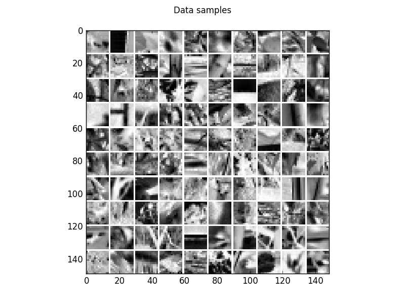
Visualization of 100 examples of the gray scale natural image dataset.
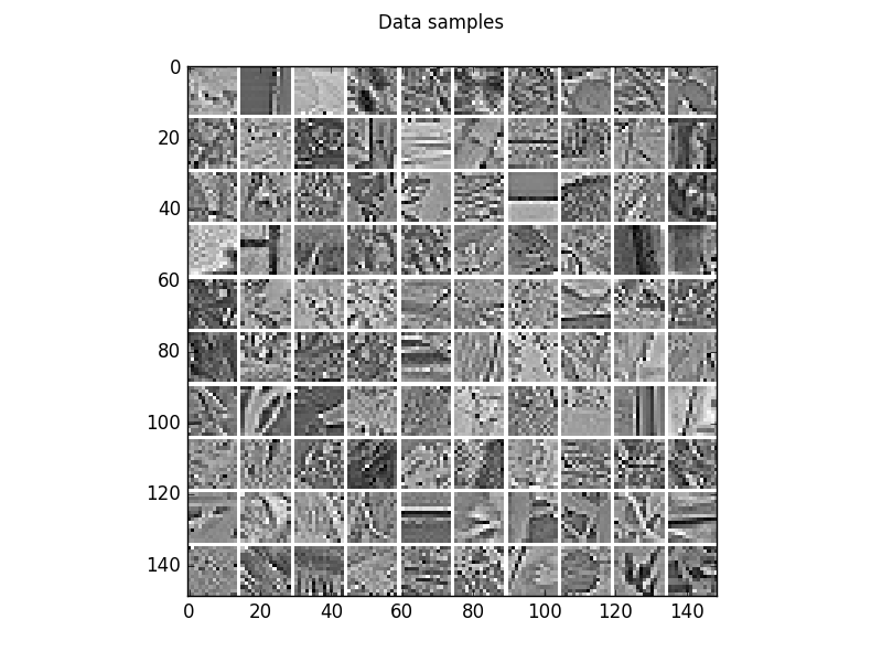
The corresponding whitened image patches.
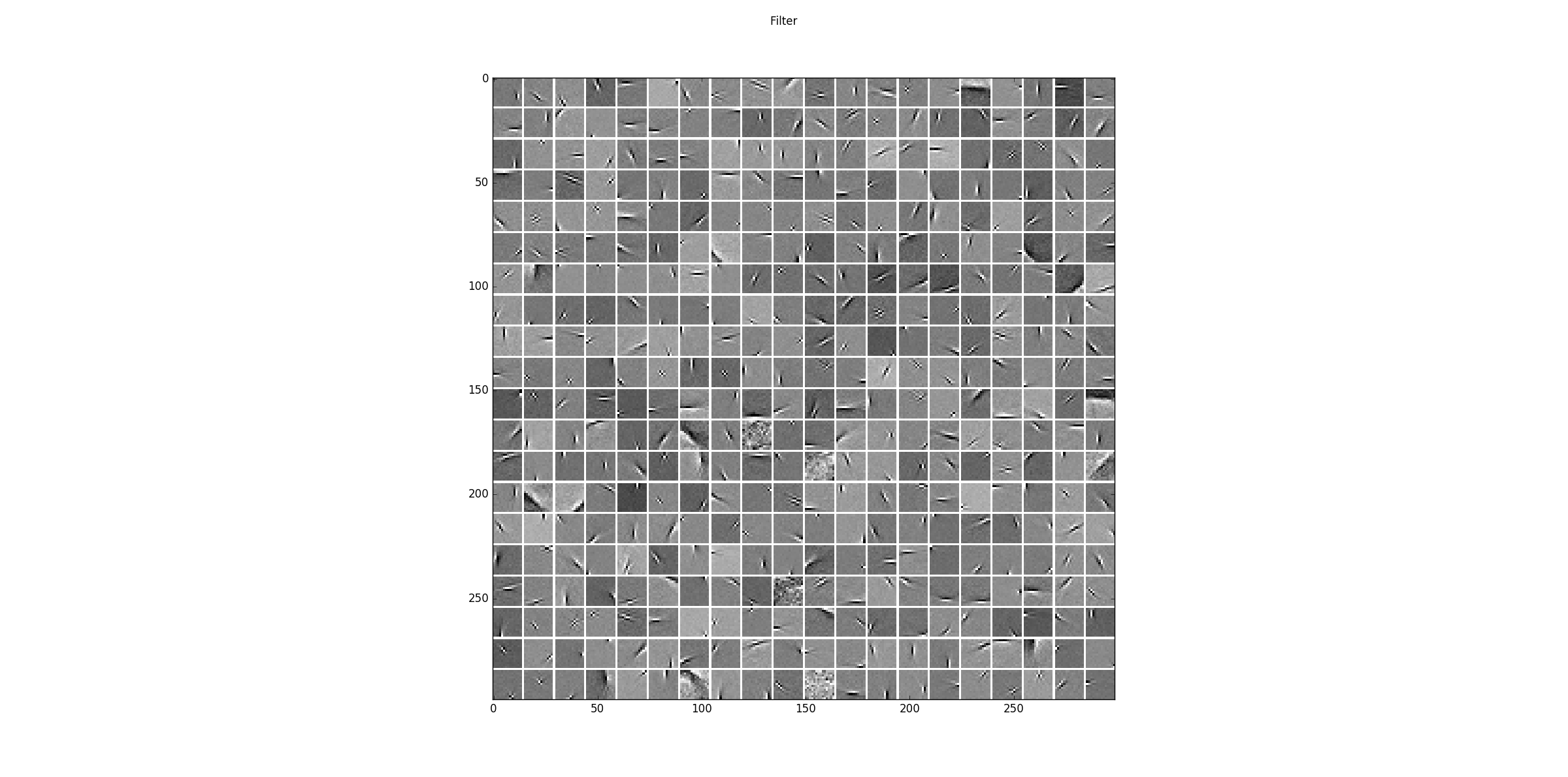
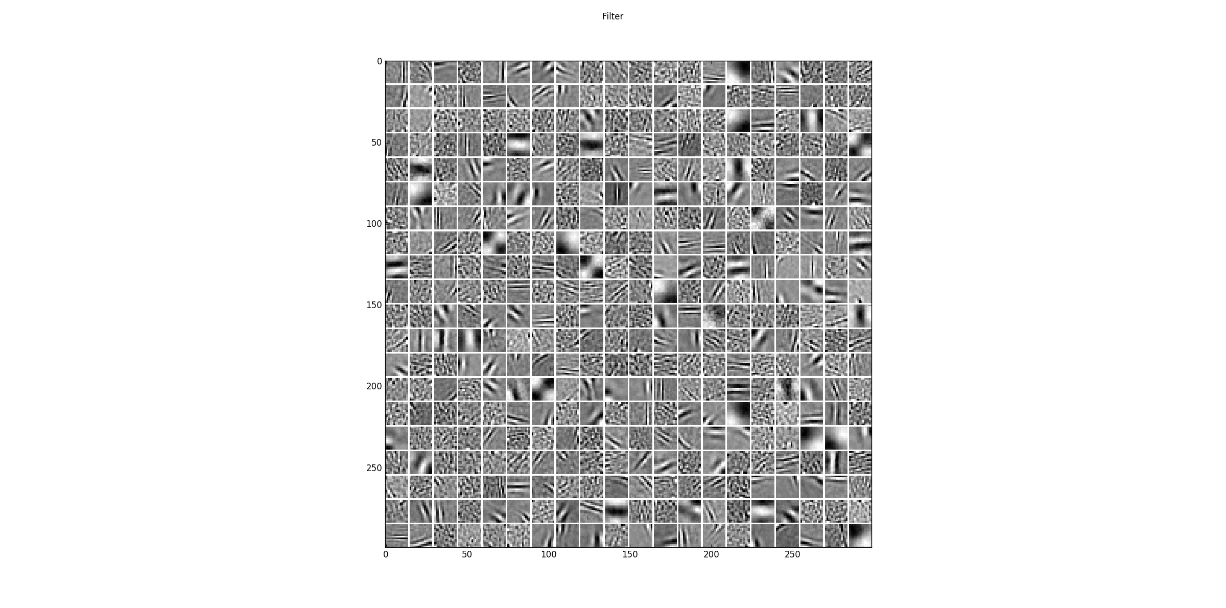
The learned filters from the whitened natural image patches.
The corresponding reconstruction of the model, that is the encoding followed by the decoding.

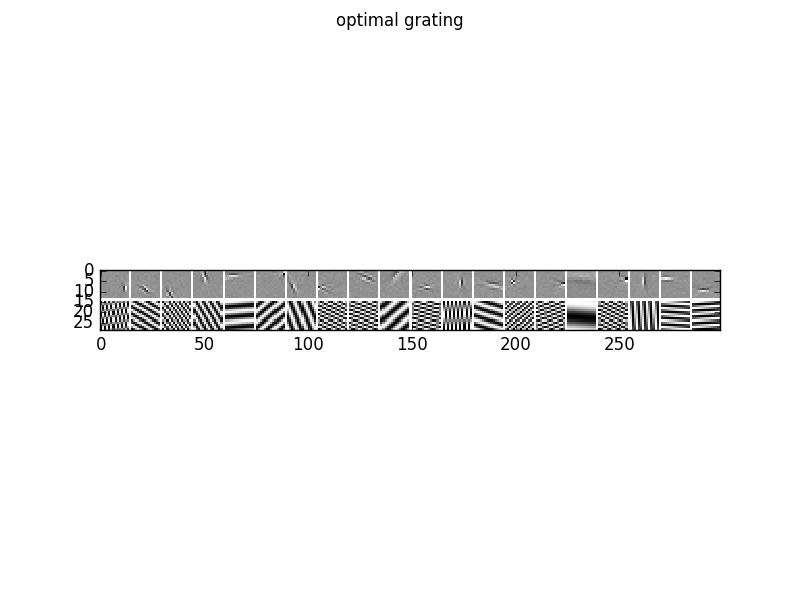
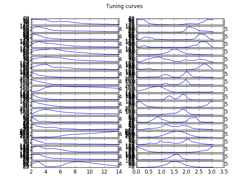
To analyze the optimal response of the learn filters we can fit a Gabor-wavelet parametrized in angle and frequency, and plot the optimal grating, here for 20 filters
as well as the corresponding tuning curves, which show the responds/activities as a function frequency in pixels/cycle (left) and angle in rad (right).
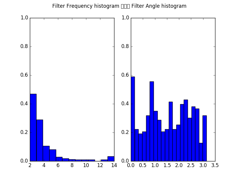
Furthermore, we can plot the histogram of all filters over the frequencies in pixels/cycle (left) and angles in rad (right).
We can also train the model on the unwhitened data leading to the following filters that cover also lower frequencies.
See also GRBM_natural_images, and ICA_natural_images.
Source code
""" Example for sparse Autoencoder (SAE) on natural image patches.

    :Version:
        1.0.0

    :Date:
        25.01.2018

    :Author:
        Jan Melchior

    :Contact:
        JanMelchior@gmx.de

    :License:

        Copyright (C) 2018 Jan Melchior

        This file is part of the Python library PyDeep.

        PyDeep is free software: you can redistribute it and/or modify
        it under the terms of the GNU General Public License as published by
        the Free Software Foundation, either version 3 of the License, or
        (at your option) any later version.

        This program is distributed in the hope that it will be useful,
        but WITHOUT ANY WARRANTY; without even the implied warranty of
        MERCHANTABILITY or FITNESS FOR A PARTICULAR PURPOSE.  See the
        GNU General Public License for more details.

        You should have received a copy of the GNU General Public License
        along with this program.  If not, see <http://www.gnu.org/licenses/>.

"""
# Import numpy, i/o functions, preprocessing, and visualization.
import numpy as numx
import pydeep.misc.io as io
import pydeep.misc.visualization as vis
import pydeep.preprocessing as pre

# Import cost functions, activation function, Autencoder and trainer module
import pydeep.base.activationfunction as act
import pydeep.base.costfunction as cost
import pydeep.ae.model as aeModel
import pydeep.ae.trainer as aeTrainer

# Set random seed
numx.random.seed(42)

# Load data (download is not existing)
data = io.load_natural_image_patches('NaturalImage.mat')

# Remove mean individually
data = pre.remove_rows_means(data)

# Shuffle data
data = numx.random.permutation(data)

# Specify input and hidden dimensions
h1 = 20
h2 = 20
v1 = 14
v2 = 14

# Whiten data using ZCA or change it to STANDARIZER for unwhitened results
zca = pre.ZCA(v1 * v2)
zca.train(data)
data = zca.project(data)

# Split in tarining and test data
train_data = data[0:50000]
test_data = data[50000:70000]

# Set hyperparameters batchsize and number of epochs
batch_size = 10
max_epochs = 20

# Create model with sigmoid hidden units, linear output units, and squared error.
ae = aeModel.AutoEncoder(v1*v2,
                         h1*h2,
                         data = train_data,
                         visible_activation_function = act.Identity(),
                         hidden_activation_function = act.Sigmoid(),
                         cost_function = cost.SquaredError(),
                         initial_weights = 0.01,
                         initial_visible_bias = 0.0,
                         initial_hidden_bias = -2.0,
# Set initially the units to be inactive, speeds up learning a little bit
                         initial_visible_offsets = 0.0,
                         initial_hidden_offsets = 0.02,
                         dtype = numx.float64)

# Initialized gradient descent trainer
trainer = aeTrainer.GDTrainer(ae)

# Train model
print 'Training'
print 'Epoch\tRE train\t\tRE test\t\t\tSparsness train\t\tSparsness test '
for epoch in range(0,max_epochs+1,1) :

    # Shuffle data
    train_data = numx.random.permutation(train_data)

    # Print reconstruction errors and sparseness for Training and test data
    print epoch, ' \t\t', numx.mean(ae.reconstruction_error(train_data)), \
        ' \t', numx.mean(ae.reconstruction_error(test_data)),\
        ' \t', numx.mean(ae.encode(train_data)), \
        ' \t', numx.mean(ae.encode(test_data))
    for b in range(0,train_data.shape[0],batch_size):

        trainer.train(data = train_data[b:(b+batch_size),:],
                      num_epochs=1,
                      epsilon=0.1,
                      momentum=0.0,
                      update_visible_offsets=0.0,
                      update_hidden_offsets=0.01,
                      reg_L1Norm=0.0,
                      reg_L2Norm=0.0,
                      corruptor=None,
                      # Rather strong sparsity regularization
                      reg_sparseness = 2.0,
                      desired_sparseness=0.001,
                      reg_contractive=0.0,
                      reg_slowness=0.0,
                      data_next=None,
# The gradient restriction is important for fast learning, see also GRBMs
                      restrict_gradient=0.1,
                      restriction_norm='Cols')

# Show filters/features
filters = vis.tile_matrix_rows(ae.w, v1,v2,h1,h2, border_size = 1,
                               normalized = True)
vis.imshow_matrix(filters, 'Filter')

# Show samples
samples = vis.tile_matrix_rows(train_data[0:100].T, v1,v2,10,10,
                               border_size = 1,normalized = True)
vis.imshow_matrix(samples, 'Data samples')

# Show reconstruction
samples = vis.tile_matrix_rows(ae.decode(ae.encode(train_data[0:100])).T,
                               v1,v2,10,10, border_size = 1,
                               normalized = True)
vis.imshow_matrix(samples, 'Reconstructed samples')

# Get the optimal gabor wavelet frequency and angle for the filters
opt_frq, opt_ang = vis.filter_frequency_and_angle(ae.w, num_of_angles=40)

# Show some tuning curves
num_filters =20
vis.imshow_filter_tuning_curve(ae.w[:,0:num_filters], num_of_ang=40)

# Show some optima grating
vis.imshow_filter_optimal_gratings(ae.w[:,0:num_filters],
                                   opt_frq[0:num_filters],
                                   opt_ang[0:num_filters])

# Show histograms of frequencies and angles.
vis.imshow_filter_frequency_angle_histogram(opt_frq=opt_frq,
                                            opt_ang=opt_ang,
                                            max_wavelength=14)

# Show all windows.
vis.show()