Independent Component Analysis on a natural image patches

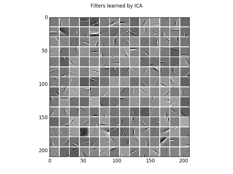
Example for Independent Component Analysis (ICA) on natural image patches. The independent components (columns of the ICA projection matrix) of natural image patches are edge detector filters.

Theory

If you are new on ICA and blind source separation, first see ICA_2D_example.

For a comparison of ICA and GRBMs on natural image patches see Gaussian-binary restricted Boltzmann machines for modeling natural image statistics. Melchior et. al. PLOS ONE 2017.

Results

The code given below produces the following output.

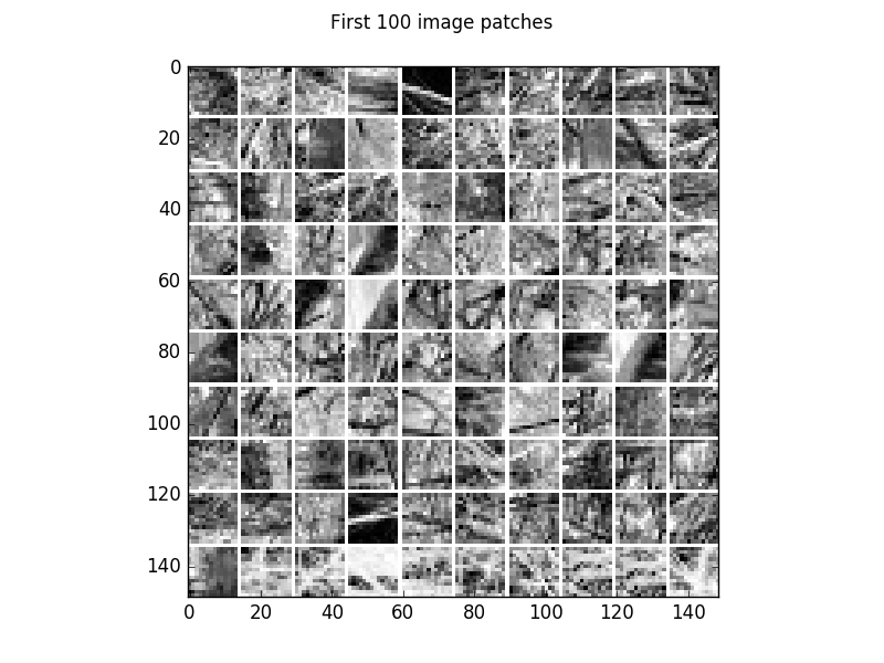
Visualization of 100 examples of the gray scale natural image dataset.

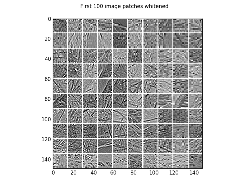
The corresponding whitened image patches.

The learned filters/independent components learned from the whitened natural image patches.

The log-likelihood on all data is:

log-likelihood on all data: -260.064878919

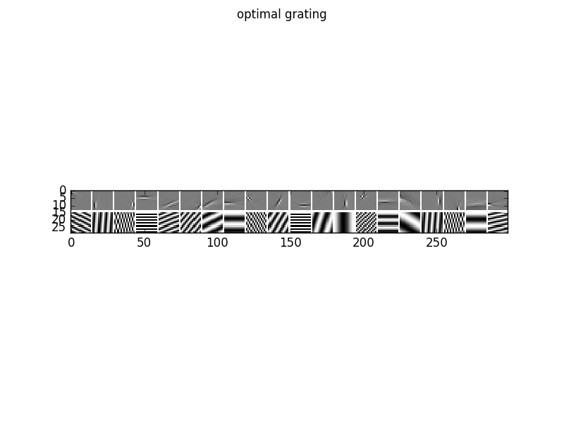
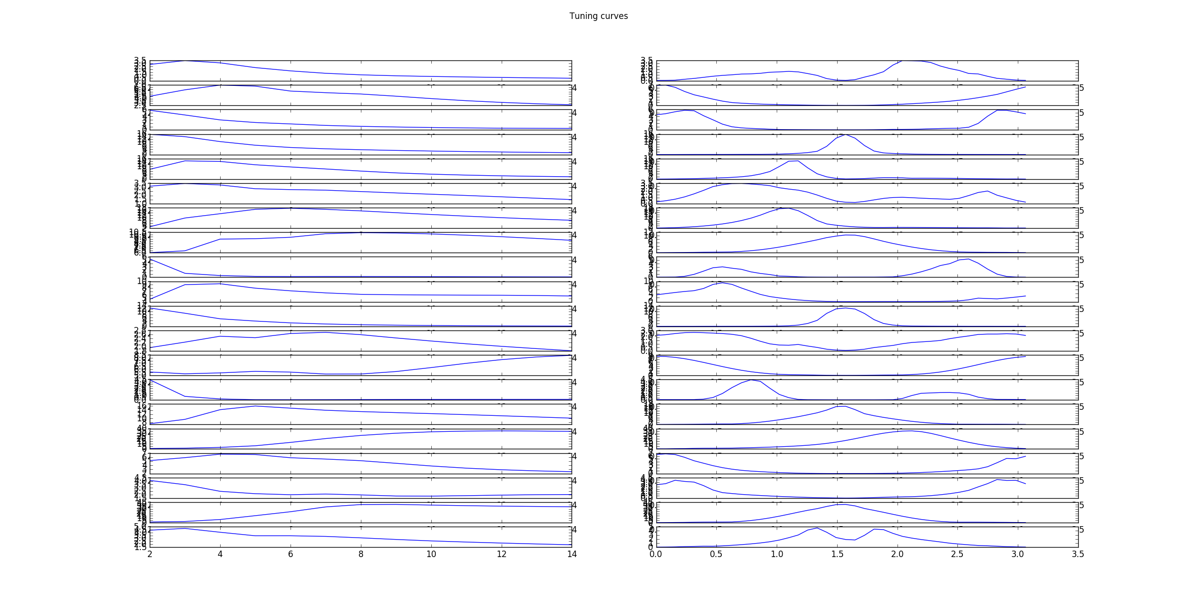
To analyze the optimal response of the learn filters we can fit a Gabor-wavelet parametrized in angle and frequency, and plot the optimal grating, here for 20 filters

as well as the corresponding tuning curves, which show the responds/activities as a function frequency in pixels/cycle (left) and angle in rad (right).

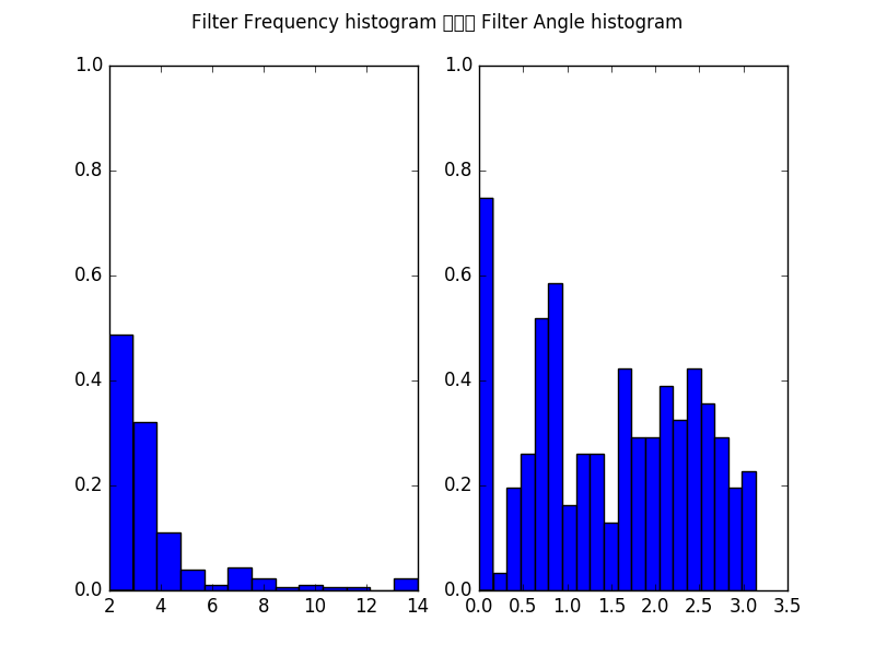
Furthermore, we can plot the histogram of all filters over the frequencies in pixels/cycle (left) and angles in rad (right).

See also GRBM_natural_images. and AE_natural_images.

Source code

""" Example for the Independent Component Analysis (ICA) on natural image patches.

    :Version:
        1.1.0

    :Date:
        22.04.2017

    :Author:
        Jan Melchior

    :Contact:
        JanMelchior@gmx.de

    :License:

        Copyright (C) 2017 Jan Melchior

        This file is part of the Python library PyDeep.

        PyDeep is free software: you can redistribute it and/or modify
        it under the terms of the GNU General Public License as published by
        the Free Software Foundation, either version 3 of the License, or
        (at your option) any later version.

        This program is distributed in the hope that it will be useful,
        but WITHOUT ANY WARRANTY; without even the implied warranty of
        MERCHANTABILITY or FITNESS FOR A PARTICULAR PURPOSE.  See the
        GNU General Public License for more details.

        You should have received a copy of the GNU General Public License
        along with this program.  If not, see <http://www.gnu.org/licenses/>.

"""

# Import ZCA, ICA, numpy, input output functions, and visualization functions
import numpy as numx
from pydeep.preprocessing import ICA, ZCA
import pydeep.misc.io as io
import pydeep.misc.visualization as vis

# Set the random seed
# (optional, if stochastic processes are involved we always get the same results)
numx.random.seed(42)

# Load data (download is not existing)
data = io.load_natural_image_patches('NaturalImage.mat')

# Specify image width and height for displaying
width = height = 14

# Use ZCA to whiten the data and train it
# (you could also use PCA whitened=True + unproject for visualization)
zca = ZCA(input_dim=width * height)
zca.train(data=data)

# ZCA projects the whitened data back to the original space, thus does not
# perform a dimensionality reduction but a whitening in the original space
whitened_data = zca.project(data)

# Create a ZCA node and train it (you could also use PCA whitened=True)
ica = ICA(input_dim=width * height)
ica.train(data=whitened_data,
          iterations=100,
          convergence=1.0,
          status=True)

# Show whitened images
images = vis.tile_matrix_rows(matrix=data[0:100].T,
                              tile_width=width,
                              tile_height=height,
                              num_tiles_x=10,
                              num_tiles_y=10,
                              border_size=1,
                              normalized=True)
vis.imshow_matrix(matrix=images,
                  windowtitle='First 100 image patches')

# Show some whitened images
images = vis.tile_matrix_rows(matrix=whitened_data[0:100].T,
                              tile_width=width,
                              tile_height=height,
                              num_tiles_x=10,
                              num_tiles_y=10,
                              border_size=1,
                              normalized=True)
vis.imshow_matrix(matrix=images,
                  windowtitle='First 100 image patches whitened')

# Show the ICA filters/bases
ica_filters = vis.tile_matrix_rows(matrix=ica.projection_matrix,
                                   tile_width=width,
                                   tile_height=height,
                                   num_tiles_x=width,
                                   num_tiles_y=height,
                                   border_size=1,
                                   normalized=True)
vis.imshow_matrix(matrix=ica_filters,
                  windowtitle='Filters learned by ICA')

# Get the optimal gabor wavelet frequency and angle for the filters
opt_frq, opt_ang = vis.filter_frequency_and_angle(ica.projection_matrix,
                                                  num_of_angles=40)

# Show some tuning curves
num_filters = 20
vis.imshow_filter_tuning_curve(ica.projection_matrix[:,0:num_filters],
                               num_of_ang=40)

# Show some optima grating
vis.imshow_filter_optimal_gratings(ica.projection_matrix[:,0:num_filters],
                                   opt_frq[0:num_filters],
                                   opt_ang[0:num_filters])

# Show histograms of frequencies and angles.
vis.imshow_filter_frequency_angle_histogram(opt_frq=opt_frq,
                                            opt_ang=opt_ang,
                                            max_wavelength=14)

print("log-likelihood on all data: "+str(numx.mean(
    ica.log_likelihood(data=whitened_data))))

# Show all windows.
vis.show()