Gaussian-binary restricted Boltzmann machine on natural image patches
Example for a Gaussian-binary restricted Boltzmann machine (GRBM) on a natural image patches. The learned filters are similar to those of ICA, see also ICA_natural_images.
Theory
If you are new on GRBMs, first see GRBM_2D_example.
For a theoretical and empirical analysis of on GRBMs on natural image patches see Gaussian-binary restricted Boltzmann machines for modeling natural image statistics. Melchior et. al. PLOS ONE 2017
Results
The code given below produces the following output.
Visualization of the learned filters, which are very similar to those of ICA.
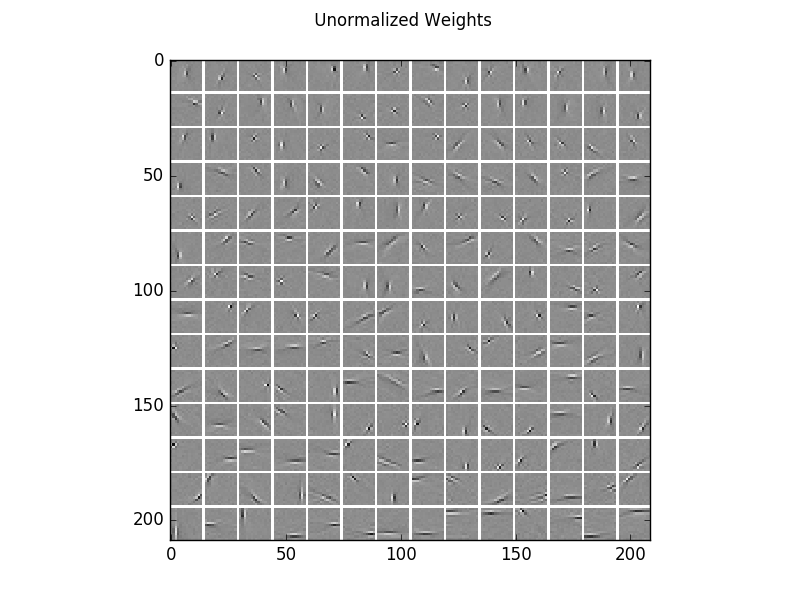
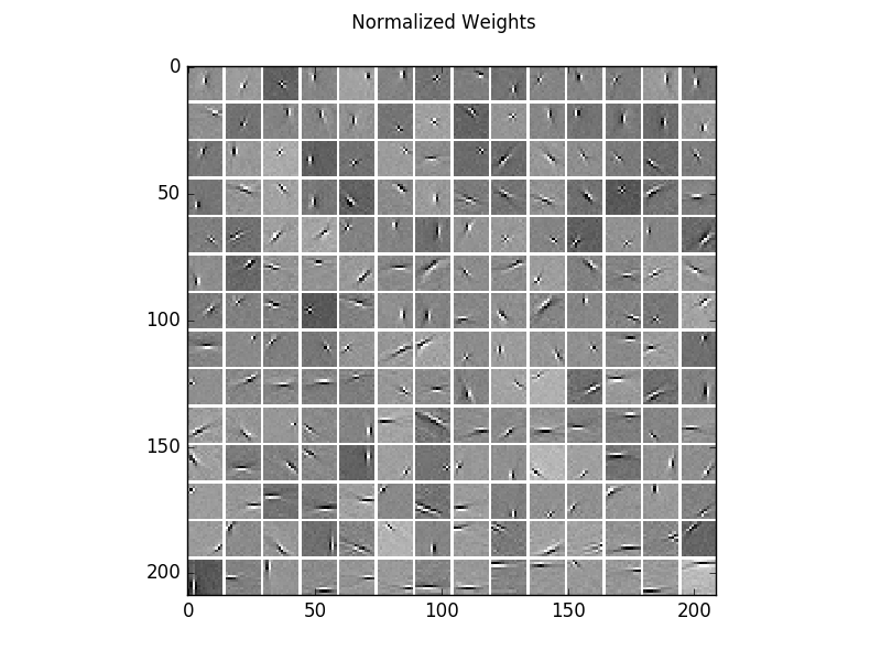
For a better visualization of the structure, here are the same filters normalized independently.
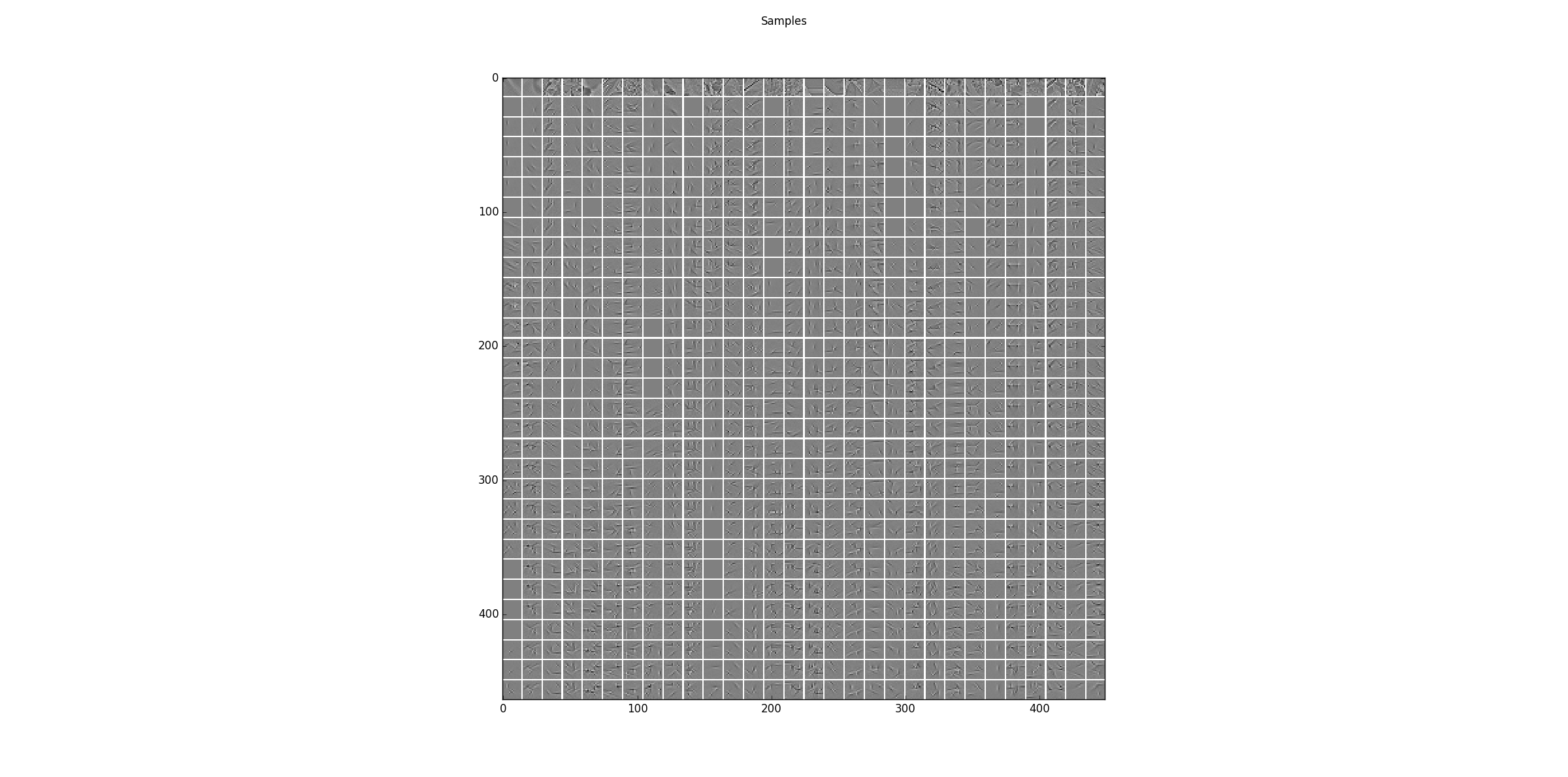
Sampling results for some examples. The first row shows some training data and the following rows are the results after one step of Gibbs-sampling starting from the previous row.
The log-likelihood and reconstruction error for training and test data
             Epoch   RE train        RE test         LL train        LL test
AIS:         200     0.73291         0.75427         -268.34107      -270.82759
reverse AIS:         0.73291         0.75427         -268.34078      -270.82731
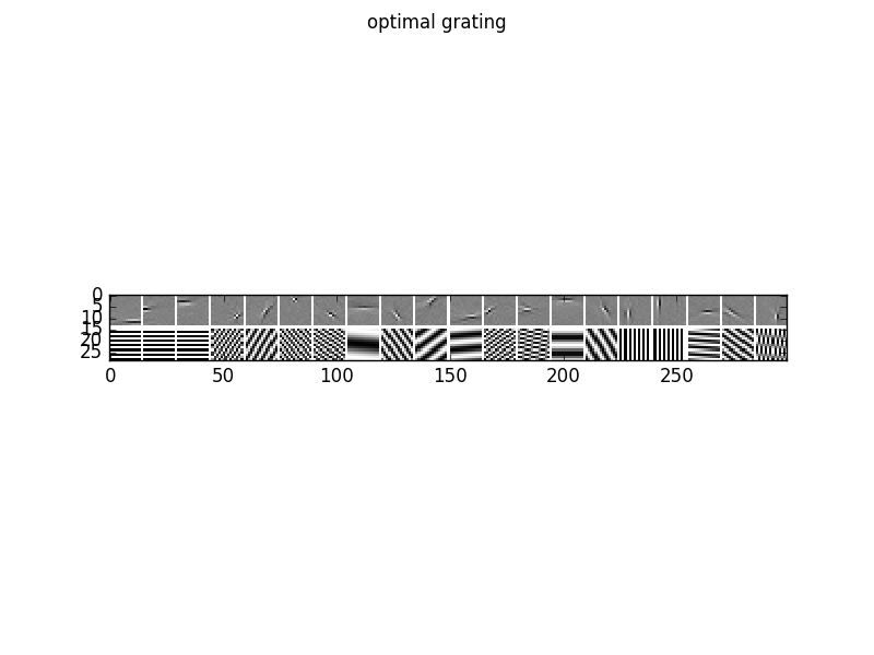
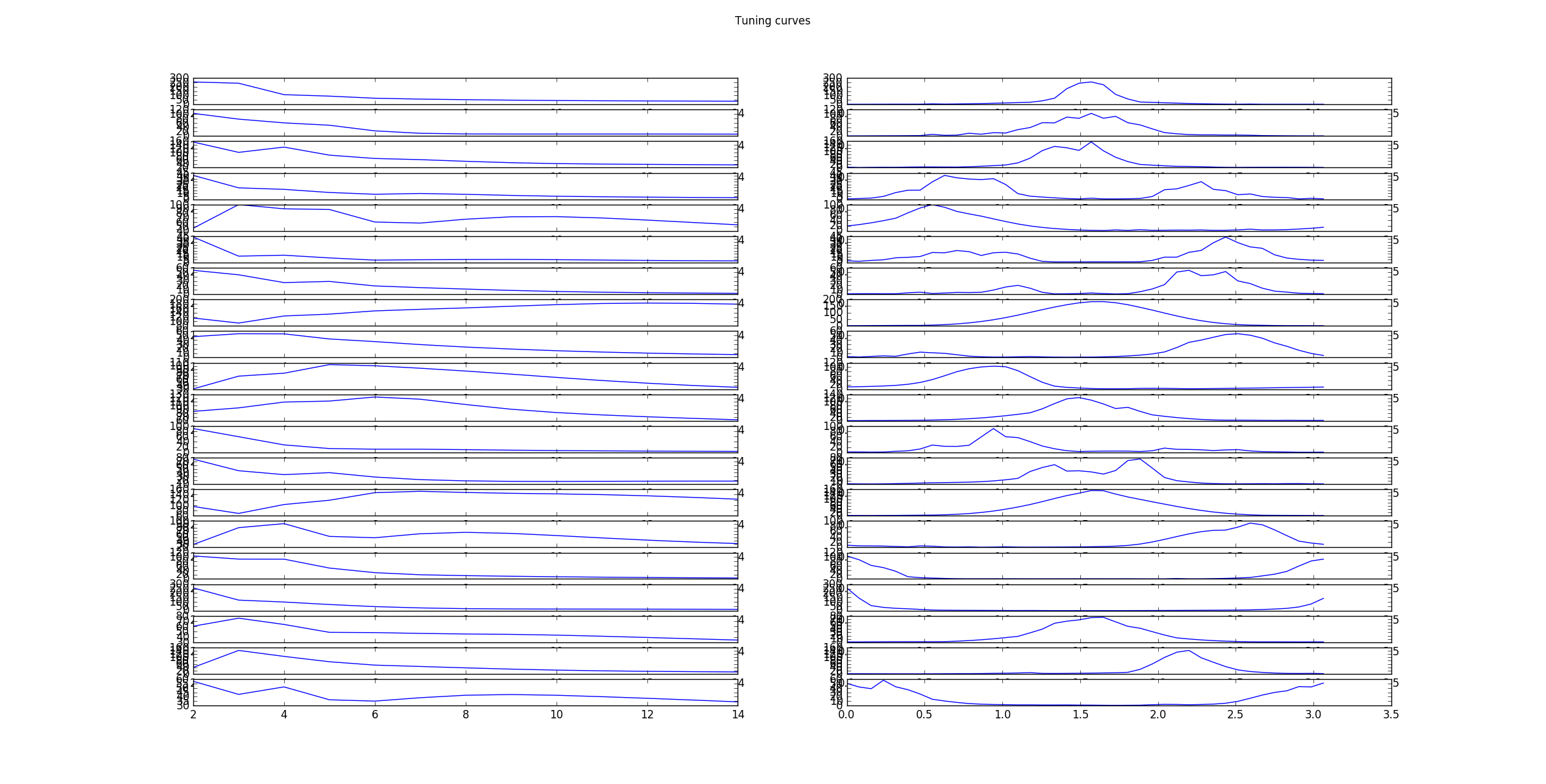
To analyze the optimal response of the learn filters we can fit a Gabor-wavelet parametrized in angle and frequency, and plot the optimal grating, here for 20 filters
as well as the corresponding tuning curves, which show the responds/activities as a function frequency in pixels/cycle (left) and angle in rad (right).
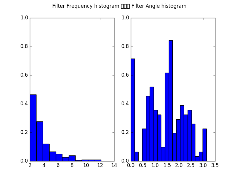
Furthermore, we can plot the histogram of all filters over the frequencies in pixels/cycle (left) and angles in rad (right).
Compare the results with thos of ICA_natural_images, and AE_natural_images..
Source code
""" Example for Gaussian-binary restricted Boltzmann machines (GRBM) on 2D data.

    :Version:
        1.1.0

    :Date:
        25.04.2017

    :Author:
        Jan Melchior

    :Contact:
        JanMelchior@gmx.de

    :License:

        Copyright (C) 2017 Jan Melchior

        This file is part of the Python library PyDeep.

        PyDeep is free software: you can redistribute it and/or modify
        it under the terms of the GNU General Public License as published by
        the Free Software Foundation, either version 3 of the License, or
        (at your option) any later version.

        This program is distributed in the hope that it will be useful,
        but WITHOUT ANY WARRANTY; without even the implied warranty of
        MERCHANTABILITY or FITNESS FOR A PARTICULAR PURPOSE.  See the
        GNU General Public License for more details.

        You should have received a copy of the GNU General Public License
        along with this program.  If not, see <http://www.gnu.org/licenses/>.

"""

# Import numpy+extensions, i/o functions, preprocessing, and visualization.
import numpy as numx
import pydeep.base.numpyextension as numxext
import pydeep.misc.io as io
import pydeep.preprocessing as pre
import pydeep.misc.visualization as vis

# Model imports: RBM estimator, model and trainer module
import pydeep.rbm.estimator as estimator
import pydeep.rbm.model as model
import pydeep.rbm.trainer as trainer

# Set random seed (optional)
# (optional, if stochastic processes are involved we get the same results)
numx.random.seed(42)

# Load data (download is not existing)
data = io.load_natural_image_patches('NaturalImage.mat')

# Remove the mean of ech image patch separately (also works without)
data = pre.remove_rows_means(data)

# Set input/output dimensions
v1 = 14
v2 = 14
h1 = 14
h2 = 14

# Whiten data using ZCA
zca = pre.ZCA(v1 * v2)
zca.train(data)
data = zca.project(data)

# Split into training/test data
train_data = data[0:40000]
test_data = data[40000:70000]

# Set restriction factor, learning rate, batch size and maximal number of epochs
restrict = 0.01 * numx.max(numxext.get_norms(train_data, axis=1))
eps = 0.1
batch_size = 100
max_epochs = 200

# Create model, initial weights=Glorot init., initial sigma=1.0, initial bias=0,
# no centering (Usually pass the data=training_data for a automatic init. that is
# set the bias and sigma to the data mean and data std. respectively, for
# whitened data centering is not an advantage)
rbm = model.GaussianBinaryVarianceRBM(number_visibles=v1 * v2,
                                      number_hiddens=h1 * h2,
                                      initial_weights='AUTO',
                                      initial_visible_bias=0,
                                      initial_hidden_bias=0,
                                      initial_sigma=1.0,
                                      initial_visible_offsets=0.0,
                                      initial_hidden_offsets=0.0,
                                      dtype=numx.float64)

# Set the hidden bias such that the scaling factor is 0.01
rbm.bh = -(numxext.get_norms(rbm.w + rbm.bv.T, axis=0) - numxext.get_norms(
    rbm.bv, axis=None)) / 2.0 + numx.log(0.01)
rbm.bh = rbm.bh.reshape(1, h1 * h2)

# Training with CD-1
k = 1
trainer_cd = trainer.CD(rbm)

# Train model, status every 10th epoch
step = 10
print('Training')
print('Epoch\tRE train\tRE test \tLL train\tLL test ')
for epoch in range(0, max_epochs + 1, 1):

    # Shuffle training samples (optional)
    train_data = numx.random.permutation(train_data)

    # Print epoch and reconstruction errors every 'step' epochs.
    if epoch % step == 0:
        RE_train = numx.mean(estimator.reconstruction_error(rbm, train_data))
        RE_test = numx.mean(estimator.reconstruction_error(rbm, test_data))
        print('%5d \t%0.5f \t%0.5f' % (epoch, RE_train, RE_test))

    # Train one epoch with gradient restriction/clamping
    # No weight decay, momentum or sparseness is used
    for b in range(0, train_data.shape[0], batch_size):
        trainer_cd.train(data=train_data[b:(b + batch_size), :],
                         num_epochs=1,
                         epsilon=[eps, 0.0, eps, eps * 0.1],
                         k=k,
                         momentum=0.0,
                         reg_l1norm=0.0,
                         reg_l2norm=0.0,
                         reg_sparseness=0,
                         desired_sparseness=None,
                         update_visible_offsets=0.0,
                         update_hidden_offsets=0.0,
                         offset_typ='00',
                         restrict_gradient=restrict,
                         restriction_norm='Cols',
                         use_hidden_states=False,
                         use_centered_gradient=False)

# Calculate reconstruction error
RE_train = numx.mean(estimator.reconstruction_error(rbm, train_data))
RE_test = numx.mean(estimator.reconstruction_error(rbm, test_data))
print '%5d \t%0.5f \t%0.5f' % (max_epochs, RE_train, RE_test)

# Approximate partition function by AIS (tends to overestimate)
logZ = estimator.annealed_importance_sampling(rbm)[0]
LL_train = numx.mean(estimator.log_likelihood_v(rbm, logZ, train_data))
LL_test = numx.mean(estimator.log_likelihood_v(rbm, logZ, test_data))
print 'AIS: \t%0.5f \t%0.5f' % (LL_train, LL_test)

# Approximate partition function by reverse AIS (tends to underestimate)
logZ = estimator.reverse_annealed_importance_sampling(rbm)[0]
LL_train = numx.mean(estimator.log_likelihood_v(rbm, logZ, train_data))
LL_test = numx.mean(estimator.log_likelihood_v(rbm, logZ, test_data))
print 'reverse AIS \t%0.5f \t%0.5f' % (LL_train, LL_test)

# Reorder RBM features by average activity decreasingly
rbmReordered = vis.reorder_filter_by_hidden_activation(rbm, train_data)

# Display RBM parameters
vis.imshow_standard_rbm_parameters(rbmReordered, v1, v2, h1, h2)

# Sample some steps and show results
samples = vis.generate_samples(rbm, train_data[0:30], 30, 1, v1, v2, False, None)
vis.imshow_matrix(samples, 'Samples')

# Get the optimal gabor wavelet frequency and angle for the filters
opt_frq, opt_ang = vis.filter_frequency_and_angle(rbm.w, num_of_angles=40)

# Show some tuning curves
num_filters =20
vis.imshow_filter_tuning_curve(rbm.w[:,0:num_filters], num_of_ang=40)

# Show some optima grating
vis.imshow_filter_optimal_gratings(rbm.w[:,0:num_filters],
                                   opt_frq[0:num_filters],
                                   opt_ang[0:num_filters])

# Show histograms of frequencies and angles.
vis.imshow_filter_frequency_angle_histogram(opt_frq=opt_frq,
                                            opt_ang=opt_ang,
                                            max_wavelength=14)

# Show all windows.
vis.show()