Independent Component Analysis on a 2D example.

Example for Independent Component Analysis (ICA) used for blind source separation on a linear 2D mixture.

Theory

If you are new on ICA and blind source separation, a good theoretical introduction is given by the Course Material in combination with the following video lectures.

and

Results

The code given below produces the following output.

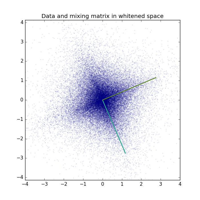
Visualization of the data and true mixing matrix projected to the whitened space.

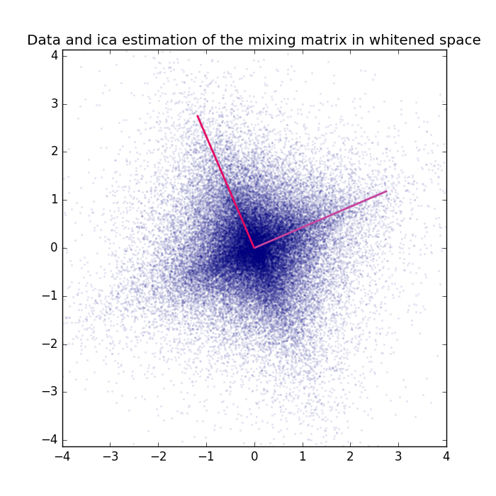
Visualization of the whitened data with the ICA projection matrix, that is the estimation of the whitened mixing matrix. Note that ICA is invariant to sign flips of the sources. The columns of the estimated mixing matrix are most likely a permutation of the columns of the original mixing matrix and can also be a 180 degrees rotated version (original vector multiplied by -1). The Amari distance is invariant to permutations and flips of the matrix columns and can thus be used to compare to mixing matrices.

Amari distanca between true mixing matrix and estimated mixing matrix: .. code-block:: Python

0.00989836830489

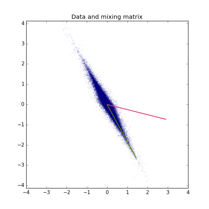
We can also project the ICA projection matrix back to the original space and compare the results in the original space.

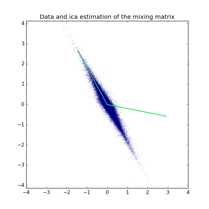
The log-likelihood on all data is:

log-likelihood on all data: -2.73863050034

For a real-world application see the ICA_natural_images example.

Source code

""" Example for the Independent Component Analysis on a 2D example.

    :Version:
        1.1.0

    :Date:
        22.04.2017

    :Author:
        Jan Melchior

    :Contact:
        JanMelchior@gmx.de

    :License:

        Copyright (C) 2017 Jan Melchior

        This file is part of the Python library PyDeep.

        PyDeep is free software: you can redistribute it and/or modify
        it under the terms of the GNU General Public License as published by
        the Free Software Foundation, either version 3 of the License, or
        (at your option) any later version.

        This program is distributed in the hope that it will be useful,
        but WITHOUT ANY WARRANTY; without even the implied warranty of
        MERCHANTABILITY or FITNESS FOR A PARTICULAR PURPOSE.  See the
        GNU General Public License for more details.

        You should have received a copy of the GNU General Public License
        along with this program.  If not, see <http://www.gnu.org/licenses/>.

"""

# Import numpy, numpy extensions, ZCA, ICA, 2D linear mixture, and visualization
import numpy as numx
import pydeep.base.numpyextension as numxext
from pydeep.preprocessing import ZCA, ICA
from pydeep.misc.toyproblems import generate_2d_mixtures
import pydeep.misc.visualization as vis

# Set the random seed
# (optional, if stochastic processes are involved we get the same results)
numx.random.seed(42)

# Create 2D linear mixture, 50000 samples, mean = 0, std = 3
data, mixing_matrix = generate_2d_mixtures(num_samples=50000,
                                           mean=0.0,
                                           scale=3.0)

# Zero Phase Component Analysis (ZCA) - Whitening in original space
zca = ZCA(data.shape[1])
zca.train(data)
whitened_data = zca.project(data)

# Independent Component Analysis (ICA)
ica = ICA(whitened_data.shape[1])

ica.train(whitened_data, iterations=100, status=False)
data_ica = ica.project(whitened_data)

# print the ll on the data
print("Log-likelihood on all data: "+str(numx.mean(
    ica.log_likelihood(data=whitened_data))))

print("Amari distanca between true mixing matrix and estimated mixing matrix: "+str(
    vis.calculate_amari_distance(zca.project(mixing_matrix.T), ica.projection_matrix.T)))

# For better visualization the principal components are rescaled
scale_factor = 3

# Display results: the matrices are normalized such that the
# column norm equals the scale factor

# Figure 1 - Data and mixing matrix
vis.figure(0, figsize=[7, 7])
vis.title("Data and mixing matrix")
vis.plot_2d_data(data)
vis.plot_2d_weights(numxext.resize_norms(mixing_matrix,
                                         norm=scale_factor,
                                         axis=0))
vis.axis('equal')
vis.axis([-4, 4, -4, 4])

# Figure 2 - Data and mixing matrix in whitened space
vis.figure(1, figsize=[7, 7])
vis.title("Data and mixing matrix in whitened space")
vis.plot_2d_data(whitened_data)
vis.plot_2d_weights(numxext.resize_norms(zca.project(mixing_matrix.T).T,
                                         norm=scale_factor,
                                         axis=0))
vis.axis('equal')
vis.axis([-4, 4, -4, 4])

# Figure 3 - Data and ica estimation of the mixing matrix in whitened space
vis.figure(2, figsize=[7, 7])
vis.title("Data and ICA estimation of the mixing matrix in whitened space")
vis.plot_2d_data(whitened_data)
vis.plot_2d_weights(numxext.resize_norms(ica.projection_matrix,
                                         norm=scale_factor,
                                         axis=0))
vis.axis('equal')
vis.axis([-4, 4, -4, 4])

# Figure 3 - Data and ica estimation of the mixing matrix
vis.figure(3, figsize=[7, 7])
vis.title("Data and ICA estimation of the mixing matrix")
vis.plot_2d_data(data)
vis.plot_2d_weights(
    numxext.resize_norms(zca.unproject(ica.projection_matrix.T).T,
                         norm=scale_factor,
                         axis=0))
vis.axis('equal')
vis.axis([-4, 4, -4, 4])



# Show all windows
vis.show()