Small binary RBM on MNIST
Example for training a centered and normal Binary Restricted Boltzmann machine on the MNIST handwritten digit dataset and its flipped version (1-MNIST). The model is small enough to calculate the exact log-Likelihood. For comparision annealed importance sampling and reverse annealed importance sampling are used for estimating the partition function.
It allows to reproduce the results from the publication How to Center Deep Boltzmann Machines. Melchior et al. JMLR 2016.
Theory
For an analysis of the advantage of centering in RBMs see How to Center Deep Boltzmann Machines. Melchior et al. JMLR 2016.
If you are new on RBMs, you can have a look into my master’s theses
A good theoretical introduction is also given by the Course Material in combination with the following video lectures.
and
Results
The code given below produces the following output.
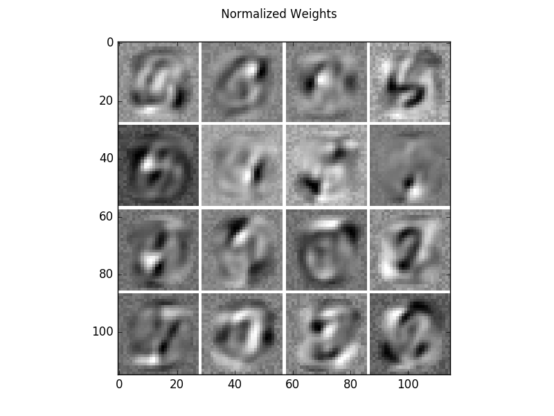
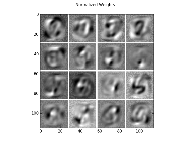
Learned filters of a centered binary RBM on the MNIST dataset. The filters have been normalized such that the structure is more prominent.
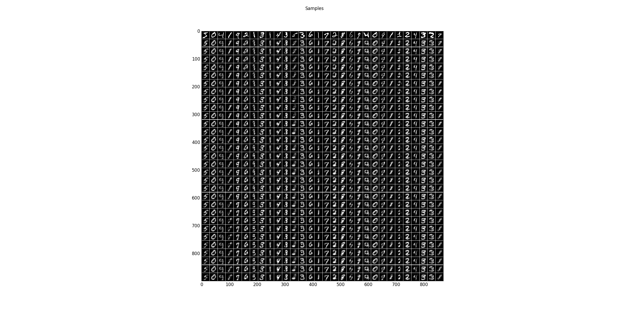
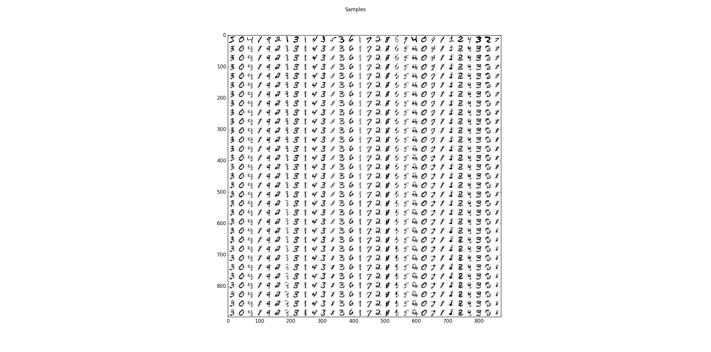
Sampling results for some examples. The first row shows the training data and the following rows are the results after one Gibbs-sampling step starting from the previous row.
The Log-Likelihood is calculated using the exact Partition function, an annealed importance sampling estimation (optimistic) and reverse annealed importance sampling estimation (pessimistic).
True Partition:         310.18444704  (LL train: -143.149739926, LL test: -142.56382054)
AIS Partition:          309.693954732 (LL train: -142.659247618, LL test: -142.073328232)
reverse AIS Partition:  316.30736142  (LL train: -149.272654305, LL test: -148.686734919)
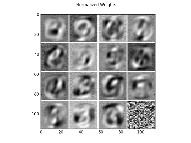
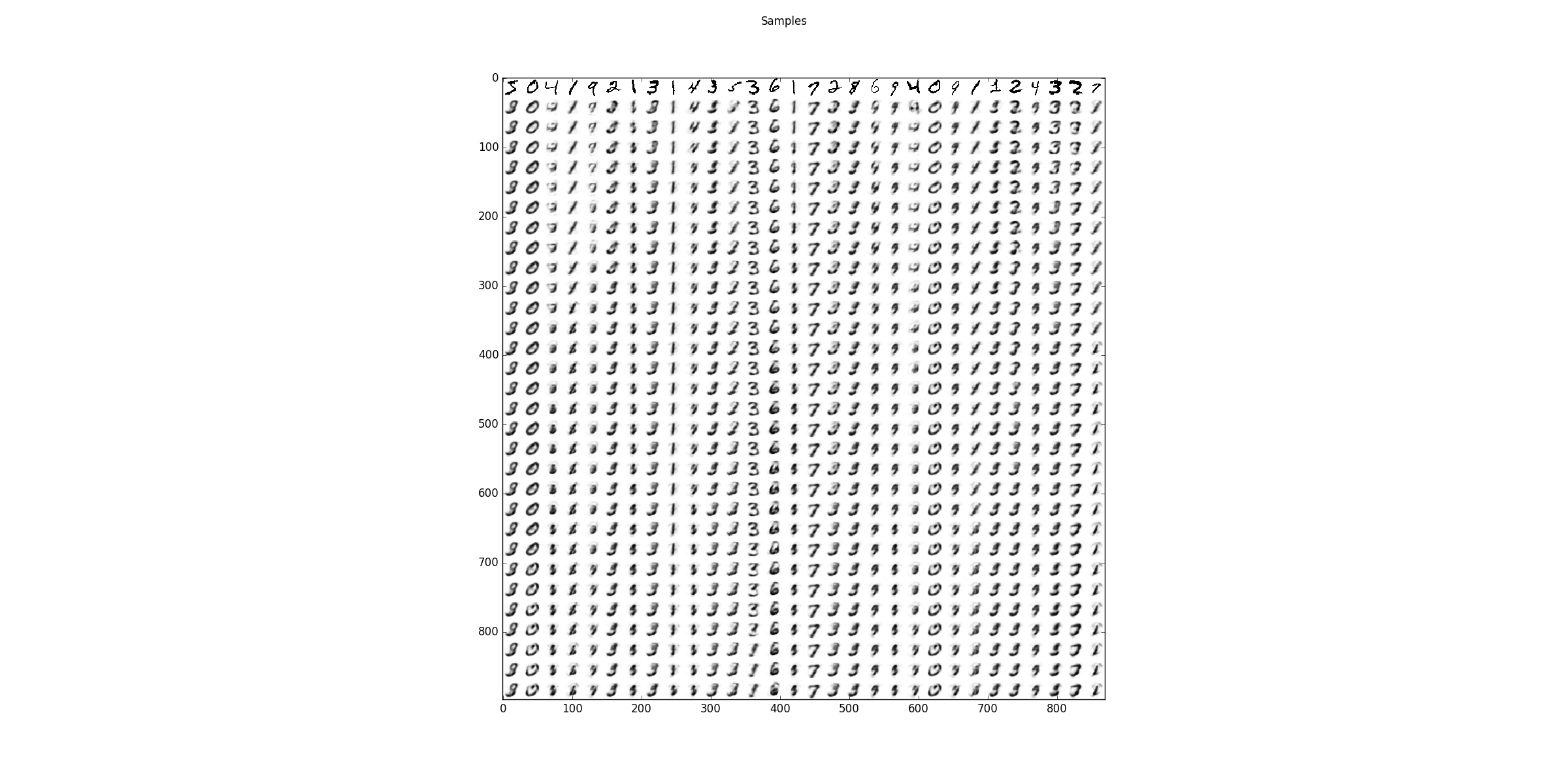
The code can also be executed without centering by setting
update_offsets = 0.0
Resulting in the following weights and sampling steps.
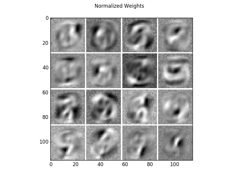
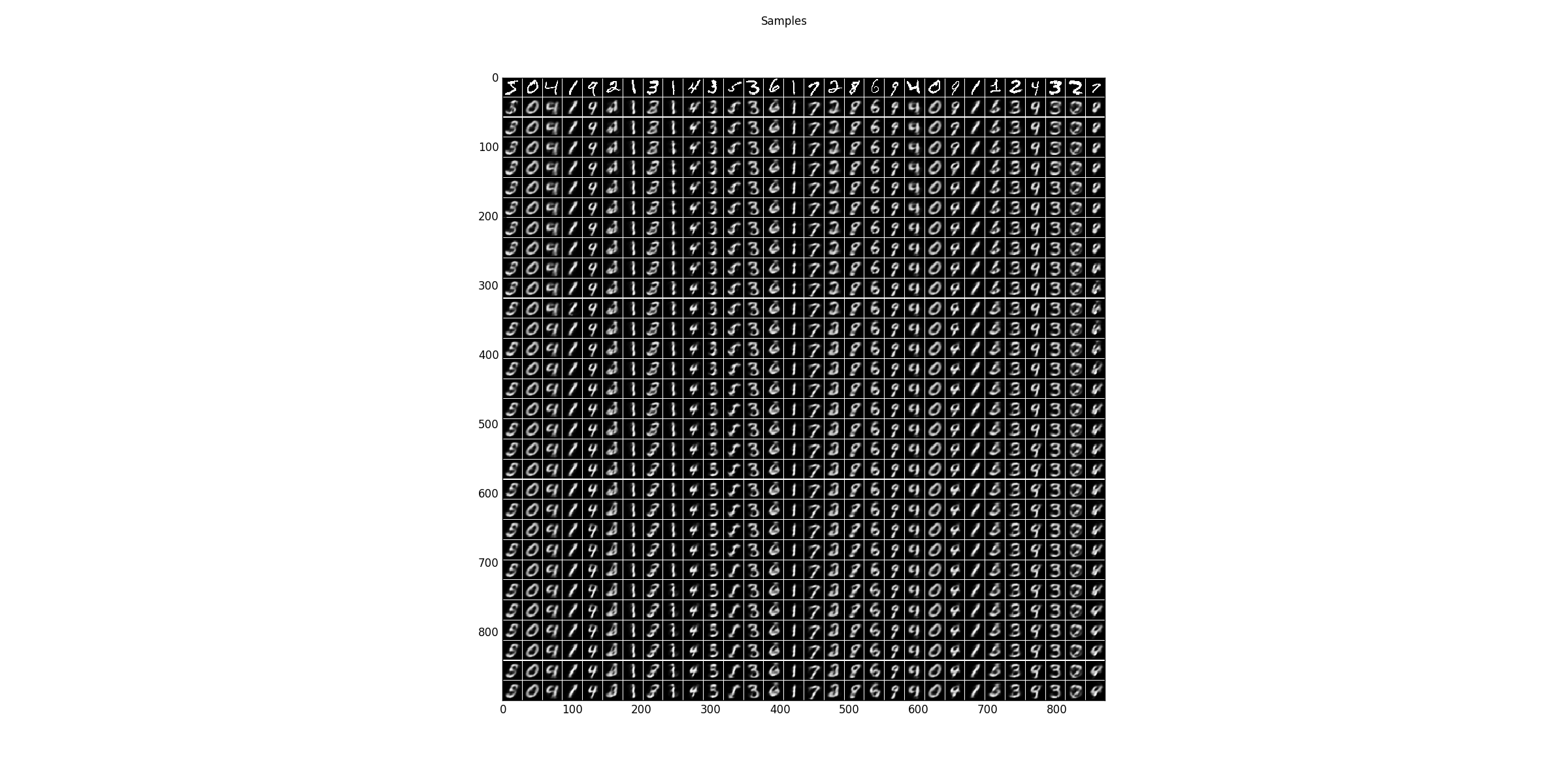
The Log-Likelihood for this model is worse (6.5 nats lower).
True Partition:         190.951945786 (LL train: -149.605105935, LL test: -149.053303204)
AIS Partition:          191.095934868 (LL train: -149.749095017, LL test: -149.197292286)
reverse AIS Partition:  191.192036843 (LL train: -149.845196992, LL test: -149.293394261)
Further, the models can be trained on the flipped version of MNIST (1-MNIST).
flipped = True
While the centered model has a similar performance on the flipped version,
True Partition:         310.245654321 (LL train: -142.812529437, LL test: -142.08692014)
AIS Partition:          311.177617039 (LL train: -143.744492155, LL test: -143.018882858)
reverse AIS Partition:  309.188366165 (LL train: -141.755241282, LL test: -141.029631984)
The normal RBM has not.
True Partition:         3495.27200694 (LL train: -183.259299994, LL test: -183.359988079)
AIS Partition:          3495.25941111 (LL train: -183.246704163, LL test: -183.347392249)
reverse AIS Partition:  3495.20117625 (LL train: -183.188469308, LL test: -183.289157393)
For a large number of hidden units see RBM_MNIST_big.
Source code
""" Example using a small BB-RBMs on the MNIST handwritten digit database.

    :Version:
        1.1.0

    :Date:
        20.04.2017

    :Author:
        Jan Melchior

    :Contact:
        JanMelchior@gmx.de

    :License:

        Copyright (C) 2017 Jan Melchior

        This file is part of the Python library PyDeep.

        PyDeep is free software: you can redistribute it and/or modify
        it under the terms of the GNU General Public License as published by
        the Free Software Foundation, either version 3 of the License, or
        (at your option) any later version.

        This program is distributed in the hope that it will be useful,
        but WITHOUT ANY WARRANTY; without even the implied warranty of
        MERCHANTABILITY or FITNESS FOR A PARTICULAR PURPOSE.  See the
        GNU General Public License for more details.

        You should have received a copy of the GNU General Public License
        along with this program.  If not, see <http://www.gnu.org/licenses/>.

"""

# model, trainer, and estimator
import pydeep.rbm.model as model
import pydeep.rbm.trainer as trainer
import pydeep.rbm.estimator as estimator

# Import numpy, input output functions, visualization, and measurement
import numpy as numx
import pydeep.misc.io as io
import pydeep.misc.visualization as vis
import pydeep.misc.measuring as mea

# Choose normal/centered RBM and normal/flipped MNIST

# normal/centered RBM --> 0.0/0.01
update_offsets = 0.01

# Flipped/Normal MNIST --> True/False
flipped = False

# Set random seed (optional)
numx.random.seed(42)

# Input and hidden dimensionality
v1 = v2 = 28
h1 = h2 = 4

# Load data (download is not existing)
train_data, _, valid_data, _, test_data, _ = io.load_mnist("mnist.pkl.gz", True)
train_data = numx.vstack((train_data, valid_data))

# Flip the dataset if chosen
if flipped:
    train_data = 1 - train_data
    test_data = 1 - test_data
    print("Flipped MNIST")
else:
    print("Normal MNIST")

# Training parameters
batch_size = 100
epochs = 50

# Create centered or normal model
if update_offsets <= 0.0:
    rbm = model.BinaryBinaryRBM(number_visibles=v1 * v2,
                                number_hiddens=h1 * h2,
                                data=train_data,
                                initial_visible_offsets=0.0,
                                initial_hidden_offsets=0.0)
    print("Normal RBM")
else:
    rbm = model.BinaryBinaryRBM(number_visibles=v1 * v2,
                                number_hiddens=h1 * h2,
                                data=train_data,
                                initial_visible_offsets='AUTO',
                                initial_hidden_offsets='AUTO')
    print("Centered RBM")

# Create trainer
trainer_pcd = trainer.PCD(rbm, num_chains=batch_size)

# Measuring time
measurer = mea.Stopwatch()

# Train model
print('Training')
print('Epoch\tRecon. Error\tLog likelihood train\tLog likelihood test\tExpected End-Time')
for epoch in range(epochs):

    # Loop over all batches
    for b in range(0, train_data.shape[0], batch_size):
        batch = train_data[b:b + batch_size, :]
        trainer_pcd.train(data=batch,
                          epsilon=0.01,
                          update_visible_offsets=update_offsets,
                          update_hidden_offsets=update_offsets)

    # Calculate Log-Likelihood, reconstruction error and expected end time every 5th epoch
    if (epoch==0 or (epoch+1) % 5 == 0):
        logZ = estimator.partition_function_factorize_h(rbm)
        ll_train = numx.mean(estimator.log_likelihood_v(rbm, logZ, train_data))
        ll_test = numx.mean(estimator.log_likelihood_v(rbm, logZ, test_data))
        re = numx.mean(estimator.reconstruction_error(rbm, train_data))
        print('{}\t\t{:.4f}\t\t\t{:.4f}\t\t\t\t{:.4f}\t\t\t{}'.format(
        epoch+1, re, ll_train, ll_test, measurer.get_expected_end_time(epoch+1, epochs)))
    else:
        print(epoch+1)

measurer.end()

# Print end/training time
print("End-time: \t{}".format(measurer.get_end_time()))
print("Training time:\t{}".format(measurer.get_interval()))

# Calculate true partition function
logZ = estimator.partition_function_factorize_h(rbm, batchsize_exponent=h1, status=False)
print("True Partition: {} (LL train: {}, LL test: {})".format(logZ,
    numx.mean(estimator.log_likelihood_v(rbm, logZ, train_data)),
    numx.mean(estimator.log_likelihood_v(rbm, logZ, test_data))))

# Approximate partition function by AIS (tends to overestimate)
logZ_approx_AIS = estimator.annealed_importance_sampling(rbm)[0]
print("AIS Partition: {} (LL train: {}, LL test: {})".format(logZ_approx_AIS,
    numx.mean(estimator.log_likelihood_v(rbm, logZ_approx_AIS, train_data)),
    numx.mean(estimator.log_likelihood_v(rbm, logZ_approx_AIS, test_data))))

# Approximate partition function by reverse AIS (tends to underestimate)
logZ_approx_rAIS = estimator.reverse_annealed_importance_sampling(rbm)[0]
print("reverse AIS Partition: {} (LL train: {}, LL test: {})".format(
    logZ_approx_rAIS,
    numx.mean(estimator.log_likelihood_v(rbm, logZ_approx_rAIS, train_data)),
    numx.mean(estimator.log_likelihood_v(rbm, logZ_approx_rAIS, test_data))))

# Reorder RBM features by average activity decreasingly
reordered_rbm = vis.reorder_filter_by_hidden_activation(rbm, train_data)

# Display RBM parameters
vis.imshow_standard_rbm_parameters(reordered_rbm, v1, v2, h1, h2)

# Sample some steps and show results
samples = vis.generate_samples(rbm, train_data[0:30], 30, 1, v1, v2, False, None)
vis.imshow_matrix(samples, 'Samples')

# Display results
vis.show()